Add Rockset Connector
1. ADDING THE ROCKSET CONNECTOR TO GRAFANA
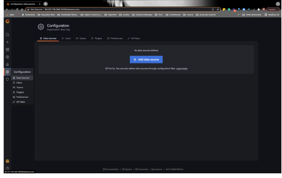
- Once you log in, go to the left nav bar, click on the gear/configurations icon and click on Add data sources:
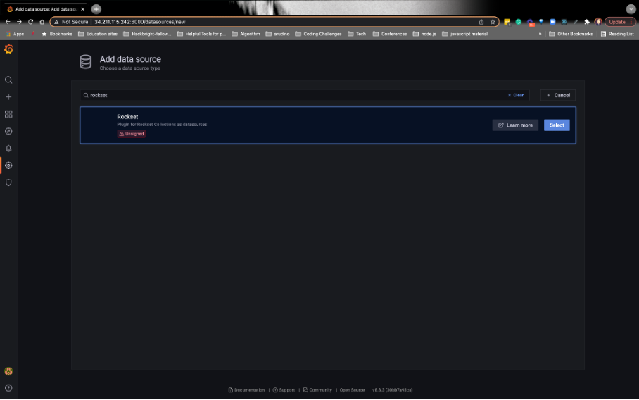
- Search for and select the Rockset connector:
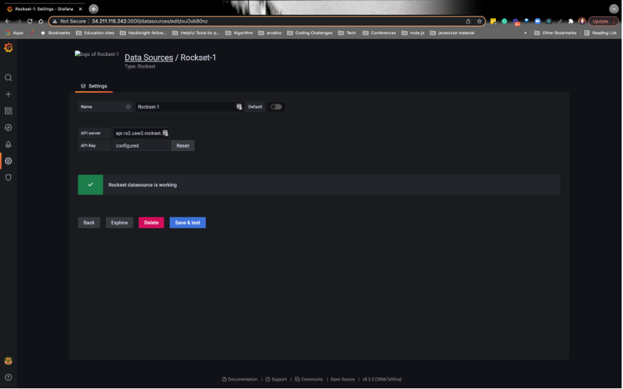
- Paste your Rockset API key from the console and click on Save & test in the bottom-right corner. Be sure to update the API server with
api.use1a1.rockset.com
2. CREATING THE GRAFANA PANEL FOR ANALYTICAL QUERY 1: Querying DynamoDB price_float field
Run this script on Cloud9, as you did in the beginning (make sure you see the script in the directory):
python scriptReadS3.pyAfter the script is running, navigate to the + icon in Grafana and click on Add a new panel:
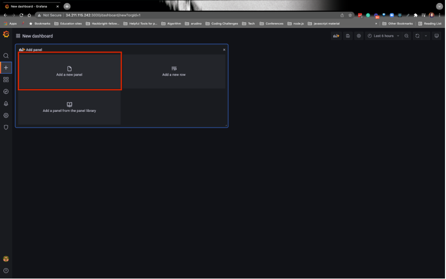
Please reference the below image.
a) In the Grafana text editor, paste the first analytical query - remember you saved it as a Query Lambda earlier.
b) For Time Column, enter timen. On the far right, choose Gauge (see the below image):
To recap, here’s our 1st query:
   SELECT
       TIME_BUCKET(days(1), c._event_time) as timen,
       AVG(c.price_float) as avgprice,
   FROM
       commons.CarPurchases as c
   WHERE
       c._event_time > :startTime AND c._event_time < :stopTime
   GROUP BY
       timen
   ORDER BY
       timen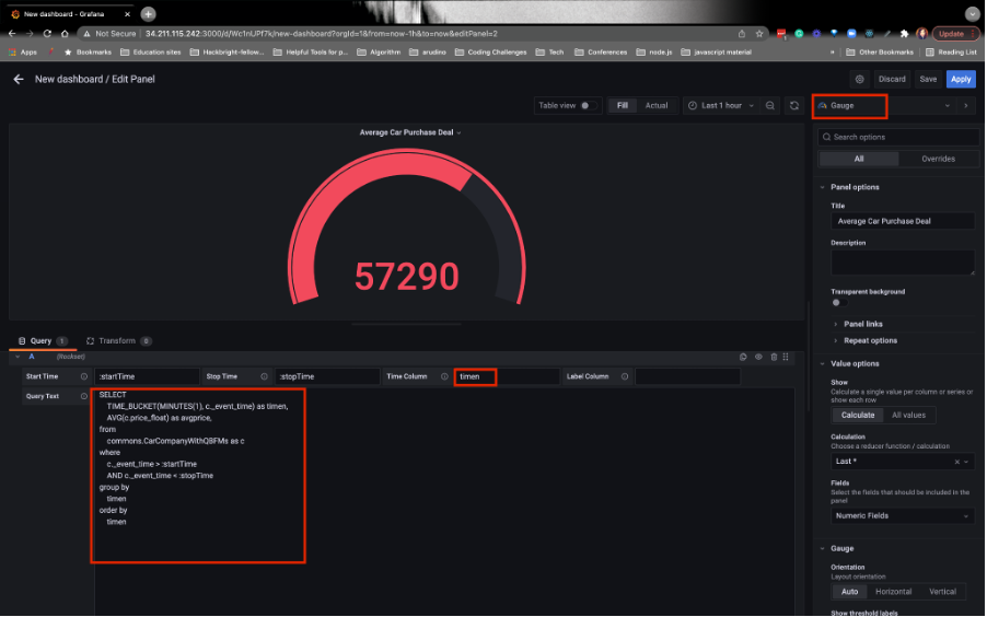
- Edit the timestamp on Grafana to be UTC. Click on the drop-down where you see the timestamp:
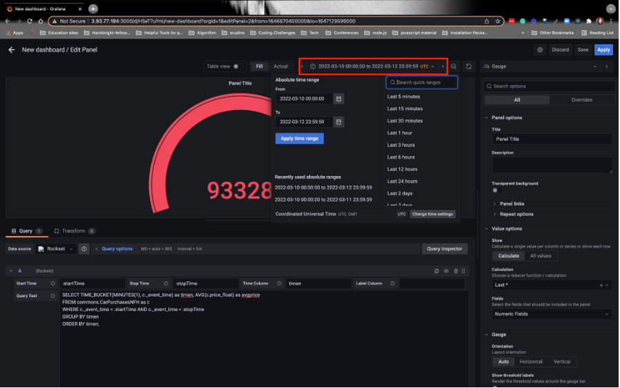
- See image below:
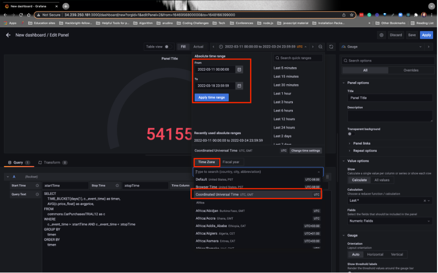
- Choose today’s date on the From calendar.
- Choose a week later on the To calendar.
- Choose UTC as a timestamp option (when you run the query on Rockset, you’ll see the timestamp, 2022-03-30 if you’re attending the live workshop):
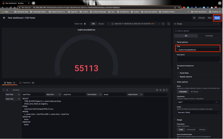
It might take a few seconds for the visualization to show up– don’t worry if it doesn’t show up immediately.
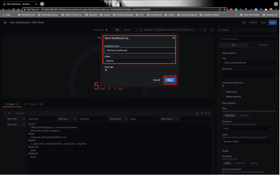
Name the panel AvgPurchaseByMinute. Then, Apply the changes:
Finally, click Save on the upper right [not shown]. Save the dashboard as Real-time Dashboard:
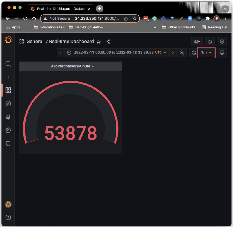
Set the refresh period to 1m. You should see the numbers updating live on Grafana every minute. If it doesn’t show up immediately, don’t panic– it may take a few minutes for it to initially load!
3. VISUALIZATION FOR ANALYTICAL QUERY 2: JOINing DynamoDB and S3 data
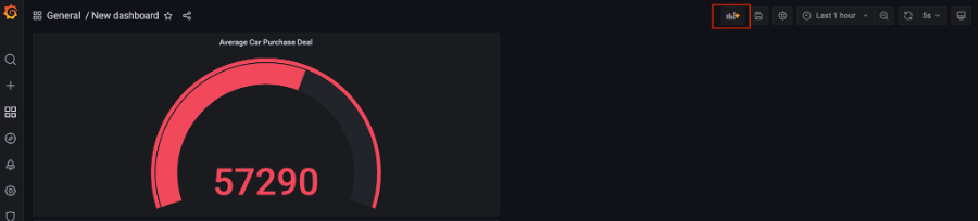
- For our second analytical query, and moving forward, we’re going to hit the +graph icon and then click Add a new panel:
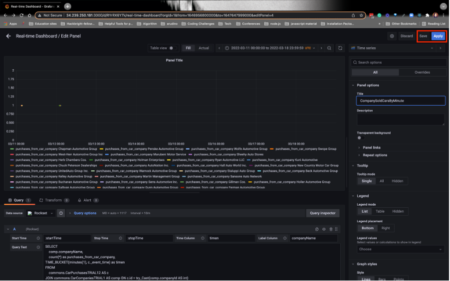
Copy the second analytical query you wrote and paste it into the Grafana editor. As a reminder, the query you’re pasting is this:
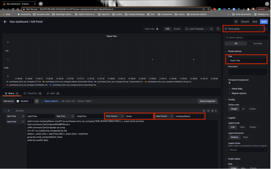
   SELECT
       comp.companyName,
       count(*) as purchases_from_car_company,
       TIME_BUCKET(MINUTES(1), c._event_time) as timen
   FROM
       commons.CarPurchases AS c
       JOIN commons.CarCompanies AS comp ON c.id = try_Cast(comp.companyId AS int)
   WHERE
       c._event_time > :startTime AND c._event_time < :stopTime
   GROUP BY
       comp.companyName,
       timen
   ORDER BY
       count(*) DESC;
Refer to the image below:
- Search for the Time Series visualization chart
- For the Time Column enter timen
- For the Label Column, enter companyName
- Rename the chart CompanySoldCarsByMinute
Note- we don’t have to update the timestamp to be UTC on the second panel because that setting is already applied.
- Click on Apply and Save. You should see the visualization look something like this:
- You should have 2 panels in your dashboard:
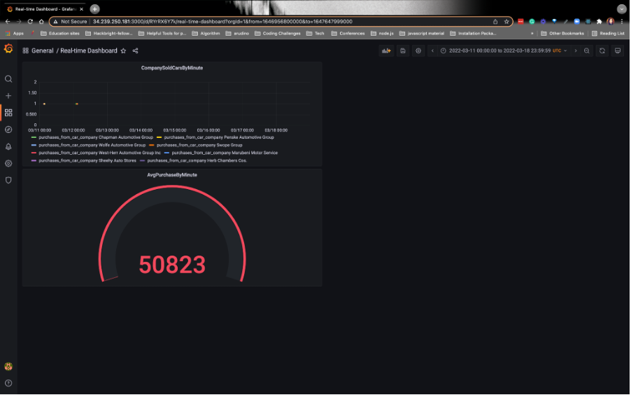
Congrats! You’ve built a real-time reporting dashboard. This marks the end of the first part of the workshop.